Asset Graph Correlation
Graph Theory Approach to Market Analysis & it's Topology
Multi-Asset Analysis via Graph Theory
Table of Contents
1. Abstract
The objective of our work is to analyze the historical prices of multiple financial symbols through the lens of graph theory. By transforming time-series price data into a network structure, we move beyond traditional isolated asset analysis. This approach allows us to visualize hidden relationships, identify clusters of symbols that move in lockstep, and uncover the broader topological structure of market dynamics.
2. Graph Theory Approach
To model the market, we utilize a simple graph. Mathematically, a simple graph is an undirected graph with no self-loops (a node connecting to itself) and no multiple edges between the same pair of nodes.
It is defined formally as: \(G = (V, E)\)
- Vertices ($V$): The set of nodes, where each node $v_i \in V$ represents a distinct financial symbol in our dataset (e.g., a specific stock, bond, or commodity ticker).
- Edges ($E$): The set of unweighted links connecting the nodes.
How We Build Our Graph:
- First, we calculate the pairwise correlation of historical price returns for all symbols in our universe.
- Next, we define a strict correlation threshold, $\tau$.
- We populate the edge set $E$ by drawing an edge $e_{ij}$ between symbol $v_i$ and symbol $v_j$ if and only if their calculated correlation is strictly greater than the threshold $correlation > \tau$.
This method creates a binary state: symbols are either connected or they are not. By adjusting $\tau$, we can filter out market noise and isolate only the most structurally significant relationships.
3. Graph Plane Mapping
Graph plane mapping (or graph drawing) is the mathematical challenge of translating the abstract topological structure of $G$ into a readable two-dimensional visualization.
We seek a mapping function $p$ that assigns each vertex $v_i \in V$ a coordinate vector $p_i = (x_i, y_i)$ in a 2D Euclidean space: \(p: V \rightarrow \mathbb{R}^2\)
Beyond simply mapping these points statically, our broader objective is to analyze this graph topologically and observe how its structure changes as time goes forward. By applying this mapping over rolling historical windows, we can track the evolution of market regimes, the clustering of asset classes during crises, and the shifting centrality of key financial instruments.
To achieve meaningful visual and mathematical representations of these dynamic structures, we introduce several famous layout approaches:
4. Famous Mapping Algorithms
Here is the mathematical breakdown of the primary metrics and objective functions used to plot graphs, followed by the algorithms that implement them.
1. Distance Preservation (Stress Minimization)
The most rigorous way to plot a graph is to ensure that the Euclidean distance between two nodes on the 2D plane closely matches their “graph-theoretic” distance (the shortest path between them along the edges).
The metric used here is Stress. The goal is to minimize the difference between the geometric distance $\Vert p_i - p_j \Vert$ and the ideal graph distance $d_{ij}$:
\[\text{Stress}(p) = \sum_{i < j} w_{ij} (\Vert p_i - p_j \Vert - d_{ij})^2\]Where $w_{ij}$ is a weighting factor, typically set to $1/d_{ij}^2$ to heavily penalize distortions between nodes that should be close together.
2. Energy Minimization (Force-Directed)
Instead of calculating exact distances, this approach models the graph as a physical system of springs and electrical charges. The metric is the total potential energy of the system, which the algorithm seeks to minimize.
It relies on two competing forces:
- Attractive Force (Springs): Pulls connected nodes together. Hooke’s Law is often used, minimizing energy proportional to the squared distance: \(U_{attr} = \sum_{(i,j) \in E} \frac{1}{2} k \Vert p_i - p_j \Vert^2\)
- Repulsive Force (Charges): Pushes all nodes apart to prevent overlap, acting like Coulomb’s law: \(U_{rep} = \sum_{i \neq j} \frac{c}{\Vert p_i - p_j \Vert}\)
The algorithm calculates the gradient of these forces and iteratively moves nodes until the system reaches an equilibrium (a local minimum of energy).
3. Spectral Metrics (Algebraic Graph Theory)
Spectral methods rely on the linear algebra of the graph’s Adjacency Matrix ($A$) and Degree Matrix ($D$). They use the Graph Laplacian, defined as:
\[L = D - A\]The mathematical objective is to place connected nodes as close together as possible, but with a constraint that prevents all nodes from collapsing into a single point (the coordinates must be orthogonal and centered at the origin). This is framed as minimizing the trace of the Laplacian matrix scaled by the position matrix $P$:
\[\min_P \text{Tr}(P^T L P) \quad \text{subject to} \quad P^T P = I\]The solution to this optimization problem simply requires finding the eigenvectors corresponding to the smallest non-zero eigenvalues of the Laplacian matrix.
I. Fruchterman-Reingold
1. The Philosophy: Physics as a Metaphor The philosophy of the Fruchterman-Reingold algorithm is rooted in particle physics and mechanics. It treats the graph as a physical system attempting to reach a state of equilibrium (minimum potential energy). It relies on two competing physical forces:
- Repulsion (Electrostatics): Every single node (asset) in the network acts like a positively charged particle. They naturally repel all other nodes. This ensures that assets do not sit on top of each other and spread out to fill the available space.
- Attraction (Springs): The edges (correlations above your threshold) act like steel springs connecting specific nodes. Hooke’s Law applies here: the further apart two connected nodes are, the harder the spring pulls them back together.
2. The Mathematics To compute the layout, the algorithm first defines an optimal distance ($k$) that should ideally exist between all nodes, based on the total area available ($A$) and the number of vertices ($\vert{}V\vert{}$), scaled by a constant $C$:
\[k = C \sqrt{\frac{A}{\vert{}V\vert{}}}\]Using the Euclidean distance ($d$) between any two nodes, the algorithm calculates the two competing forces:
-
Attractive Force ($f_a$): Applied only between nodes that share an edge. It scales quadratically with distance. \(f_a(d) = \frac{d^2}{k}\)
-
Repulsive Force ($f_r$): Applied between all pairs of nodes. It scales inversely with distance. \(f_r(d) = -\frac{k^2}{d}\)
3. The Algorithm (How It Works) To translate the math into a final 2D plot, the algorithm runs through a continuous simulation loop until it reaches a stable state:
- Initialization: Every asset is assigned a random $(x, y)$ coordinate on the 2D plane.
- Calculate Repulsion: The algorithm loops through every pair of assets. It calculates the repulsive force $f_r$ pushing them apart and stores the resulting displacement vector.
- Calculate Attraction: The algorithm loops through only the connected edges (correlations passing your threshold). It calculates the attractive spring force $f_a$ and adds this to the displacement vectors of the connected nodes.
- Position Update: Each asset is moved according to its net displacement vector (the sum of its pushes and pulls). However, the maximum distance an asset can move in a single step is strictly capped by the system’s “temperature”.
- Cooling (Simulated Annealing): The temperature is reduced slightly at the end of the iteration. The loop repeats (often 50 to 500 times) until the temperature reaches zero, preventing the nodes from oscillating and locking the assets into their final, optimal coordinates.
4. The Economic Prespective When you map a financial network using Fruchterman-Reingold, the underlying physics directly translate into fundamental market dynamics:
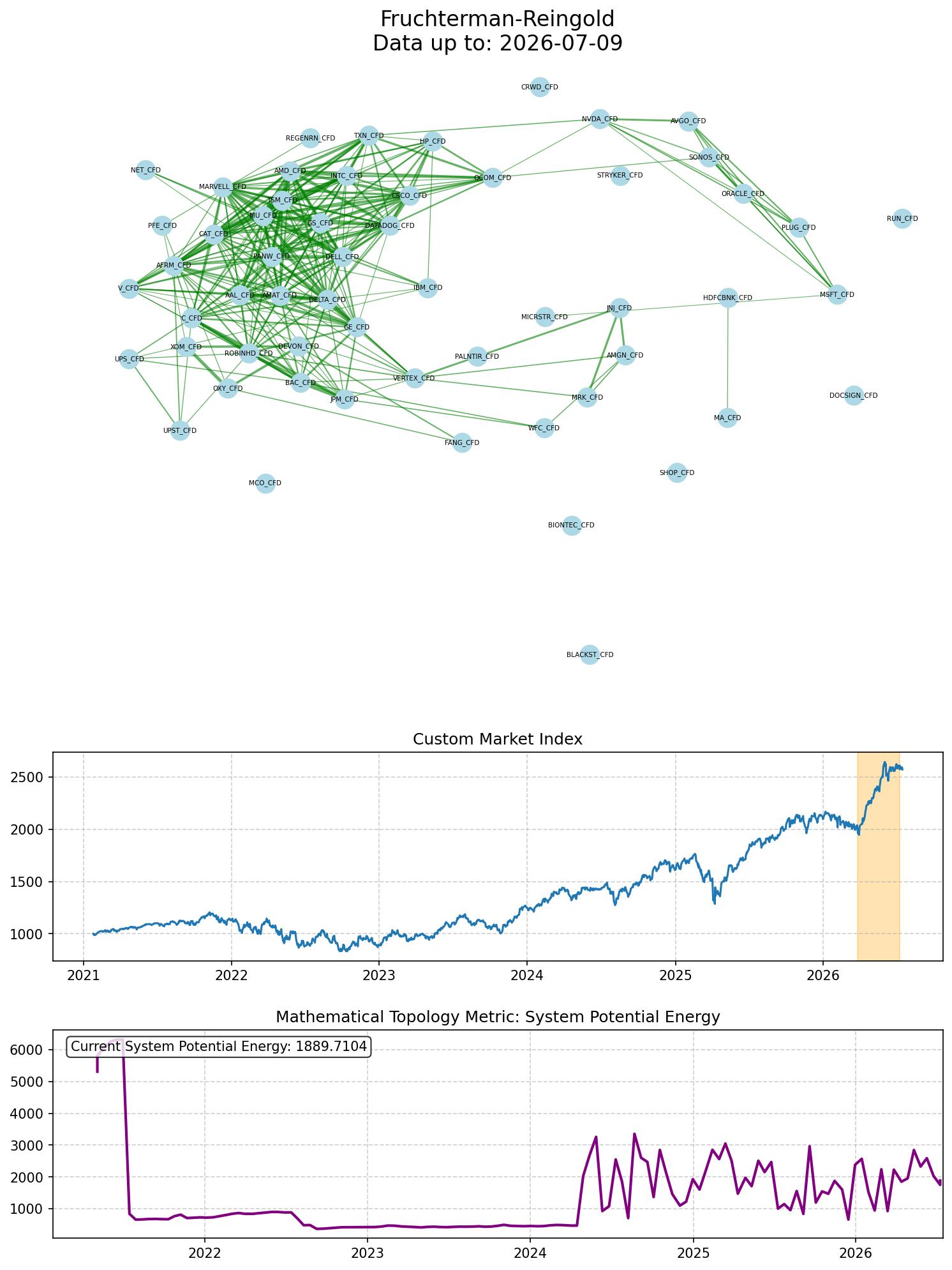
- Energy (Systemic Stress): In the algorithm, a high-energy state means the system is volatile and nodes are moving rapidly to find equilibrium. Economically, this represents systemic friction, market uncertainty, or a regime transition (like shifting from a bull to a bear market). A low-energy, settled graph represents a stable, mature market regime where assets have “priced in” their relationships.
- Repulsion (Idiosyncratic Alpha): The electrostatic repulsion represents the natural, competitive divergence of assets. If left entirely to their own fundamentals (earnings, management, product cycles), assets will chart their own course. In the network, this force pushes uncorrelated assets—like gold, sovereign bonds, and equities—far apart into distinct risk profiles, revealing your best avenues for true diversification.
- Attraction (Macro Drivers): The springs represent dominant macroeconomic drivers—such as interest rate hikes, inflation shocks, or thematic manias (e.g., the AI boom). These macro forces override individual asset fundamentals, acting as tight springs that force otherwise distinct companies to trade as a single, correlated block.
- Stability / Equilibrium (Market Pricing): The final layout of the graph is the physical equilibrium state. It is the visual representation of the market balancing idiosyncratic risk (repulsion) with systemic risk (attraction). When the graph cools and settles, you are looking at the true, underlying structure of the current financial regime.
5. Temperature & System Energy In the Fruchterman-Reingold force-directed algorithm, Temperature ($T$) dictates the maximum distance a node can move in a single iteration. It follows a simulated annealing cooling schedule. A standard exponential cooling formula at iteration $t$ is:
\[T_t = T_0 \cdot \alpha^t\]Where:
- $T_0$ is the initial temperature.
- $\alpha$ is the cooling rate (a constant $< 1$).
As $T \to 0$, the algorithm reaches an equilibrium state that minimizes the total System Potential Energy ($U$). This energy metric is the sum of the attractive spring potentials and the repulsive electrostatic potentials:
\[U = \sum_{(i,j) \in E} \frac{\|p_i - p_j\|^3}{3k} - \sum_{i \neq j} k^2 \ln(\|p_i - p_j\|)\]Where:
- $|p_i - p_j|$ is the geometric distance between nodes $i$ and $j$.
- $k$ is the optimal distance constant.
Representation of Fruchterman-Reingold Graph
II. Kamada-Kawai
1. The Philosophy: Stress Minimization and Ideal Distances The philosophy of the Kamada-Kawai algorithm is based on stress minimization. Unlike force-directed models that balance dynamic pushes and pulls, Kamada-Kawai looks for a mathematically “perfect” global layout. Its core premise is that the geometric distance between any two nodes on your 2D screen should perfectly match their theoretical “graph-theoretic” distance (the shortest path of edges between them).
It imagines the entire graph as a fully connected web of springs. Every single pair of nodes—even if they do not share a direct edge—is connected by a theoretical spring. The “ideal length” of this spring is strictly proportional to the number of steps it takes to travel between the two nodes in the actual graph.
2. The Mathematics The algorithm relies on calculating the shortest path $d_{ij}$ between all pairs of nodes $i$ and $j$ (typically using Dijkstra’s or the Floyd-Warshall algorithm).
Once the shortest paths are known, the algorithm defines the physical characteristics of the theoretical springs:
- Ideal Length ($l_{ij}$): The perfect geometric distance between two nodes, defined as $l_{ij} = L \cdot d_{ij}$, where $L$ is the desired length of a single edge.
- Spring Constant ($k_{ij}$): The stiffness of the spring. It is defined as $k_{ij} = \frac{K}{d_{ij}^2}$, where $K$ is a global constant. This means the algorithm heavily penalizes distortions between nodes that are structurally close, but is more forgiving if distant nodes are not perfectly spaced.
The objective is to minimize the total energy (or “stress”) of the entire system, $E$:
\[E = \sum_{i=1}^{\vert{}V\vert{}-1} \sum_{j=i+1}^{\vert{}V\vert{}} \frac{1}{2} k_{ij} (\Vert{}p_i - p_j\Vert{} - l_{ij})^2\]Where $\Vert{}p_i - p_j\Vert{}$ is the actual geometric distance on the 2D plane.
3. The Algorithm (How It Works) To translate this stress-minimization objective into a layout, the algorithm follows a deterministic optimization path:
- Shortest Path Calculation: It computes the shortest path between all possible pairs of assets in the network. This makes the algorithm mathematically precise but computationally heavy for massive networks.
- Initialization: It places the nodes in an initial configuration (often a circle, or utilizing another fast algorithm like Spectral Layout to get a head start).
- Gradient Calculation: It calculates the partial derivatives of the energy function $E$ for every node to find which node is currently experiencing the most “stress” (the node furthest from its ideal geometric placement).
- Node Optimization: Using a numerical method (specifically, a 2D Newton-Raphson method), it moves the single most stressed node to a local minimum of energy while freezing all other nodes.
- Iteration: It recalculates the gradients and moves the next most stressed node. This continues until the maximum stress in the entire system drops below a predefined tolerance threshold.
4. The Economic Prespective When mapping a financial correlation network using Kamada-Kawai, the focus shifts from local clusters to global macro-structure and chains of contagion:
- The Global Macro-Structure: Because Kamada-Kawai connects every node to every other node with a mathematical spring, it perfectly preserves the global shape of the market. Fruchterman-Reingold is great for seeing tight individual sectors, but Kamada-Kawai is vastly superior for understanding the grand hierarchy of asset classes (e.g., exactly how the Bond market sits in relation to the Equity market and Commodities).
- Degrees of Separation (Transmission Mechanisms): The shortest path $d_{ij}$ represents the economic chain of contagion. If an inflation shock hits Energy stocks, how many structural steps does it take for that shock to transmit to Tech stocks? Kamada-Kawai spaces assets out perfectly based on these transmission mechanisms.
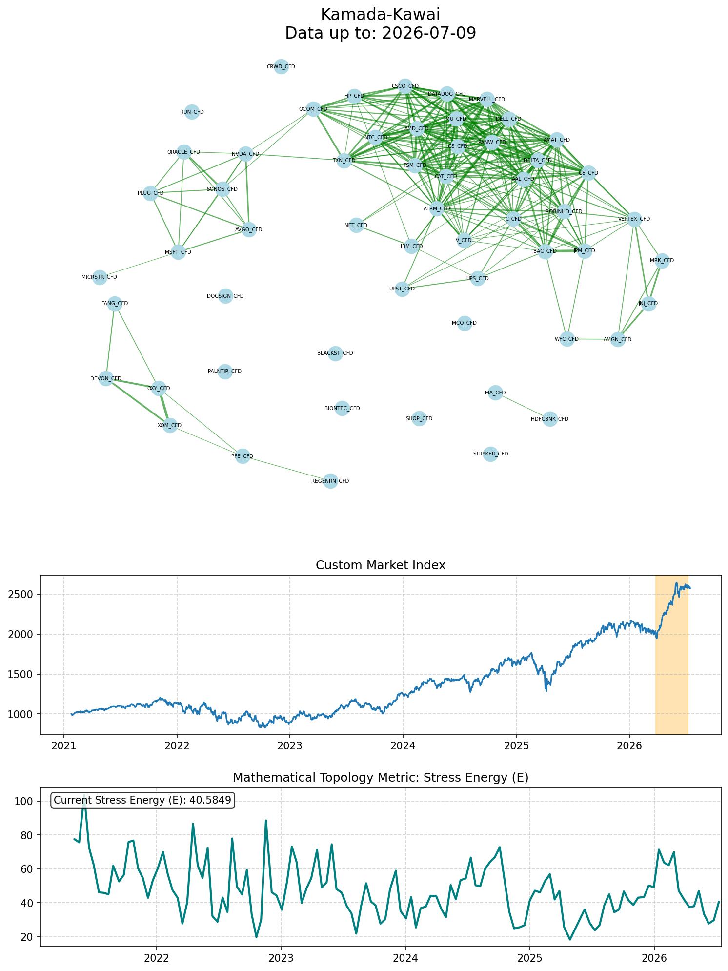
- Structural Stress (Market Dislocations): In the algorithm, “stress” occurs when nodes cannot be placed at their ideal distance. Economically, if you force this algorithm to plot a highly stressed graph over a short time window, it reveals market dislocations. It shows assets that are being forced into tighter correlations than their fundamental structure dictates—often signaling an impending mean-reversion, a pairs-trading opportunity, or a breakdown in standard market logic.
5. Total Stress Energy, $E$ The Kamada-Kawai algorithm aims to minimize the total mechanical stress ($E$) of a system of springs connecting all pairs of nodes. The objective function is:
\[E = \sum_{i=1}^{|V|-1} \sum_{j=i+1}^{|V|} \frac{1}{2} k_{ij} (\|p_i - p_j\| - l_{ij})^2\]Where:
- $|p_i - p_j|$ is the actual 2D geometric distance between nodes.
- $l_{ij} = L \cdot d_{ij}$ is the ideal geometric distance, based on the shortest graph-theoretic path ($d_{ij}$).
- $k_{ij} = \frac{K}{d_{ij}^2}$ is the spring constant (stiffness) between the nodes.
Representation of Kamada-Kawai Graph
III. Spectral Layout
Spectral layout utilizes algebraic graph theory to compute node coordinates instantly using matrix operations rather than iterative physics simulations. It relies on the Graph Laplacian matrix $L$, defined as $L = D - A$, where $D$ is the degree matrix and $A$ is the adjacency matrix.
The objective is to place connected nodes as close together as possible. Mathematically, it seeks a position matrix $P$ (containing the coordinates) that minimizes the trace of the scaled Laplacian, subject to orthogonality constraints to prevent all nodes from collapsing into the origin: \(\min_{P} \text{Tr}(P^T L P) \quad \text{subject to} \quad P^T P = I\) The optimal 2D coordinates are given by the eigenvectors corresponding to the second and third smallest eigenvalues of $L$.
III. Spectral Layout
1. The Philosophy: Algebraic Vibrations and Latent Factors The philosophy of the Spectral Layout abandons physical metaphors like springs or gravity entirely. Instead, it relies purely on algebraic graph theory and matrix decomposition. It treats the network as a mathematical object and searches for its “spectrum” (its eigenvalues and eigenvectors). Rather than pushing or pulling nodes iteratively to find a good shape, this algorithm mathematically deduces the exact inherent structure of the network in a single step, based on how the nodes partition themselves across hidden, latent mathematical dimensions.
2. The Mathematics The algorithm relies on the Graph Laplacian matrix $L$, which is defined as: \(L = D - A\) Where $D$ is the Degree Matrix (a diagonal matrix counting the number of connections each asset has) and $A$ is the Adjacency Matrix (representing the edges between assets).
The mathematical objective is to place connected nodes as close together as possible. It seeks a position matrix $P$ (containing the coordinates) that minimizes the trace of the scaled Laplacian, subject to orthogonality constraints to prevent all nodes from collapsing into the origin:
\[\min_{P} \text{Tr}(P^T L P) \quad \text{subject to} \quad P^T P = I\]The exact, mathematically optimal 2D coordinates are derived instantly by finding the eigenvectors corresponding to the second and third smallest eigenvalues of the Laplacian matrix (often related to the Fiedler vector).
3. The Algorithm (How It Works) Because it is not a physical simulation, Spectral Layout operates completely differently:
- Matrix Construction: The algorithm reads your thresholded graph and builds the Adjacency Matrix $A$ and Degree Matrix $D$, then computes the Laplacian $L$.
- Eigendecomposition: It applies linear algebra (specifically eigenvalue decomposition) to the Laplacian matrix to extract its eigenvalues and their corresponding eigenvectors.
- Coordinate Mapping: It ignores the smallest eigenvalue (which is always 0) and takes the eigenvectors of the next two smallest eigenvalues. The values in the first eigenvector become the $x$-coordinates for all assets, and the values in the second become the $y$-coordinates.
- Instant Plotting: The nodes are plotted instantly in their final, deterministic positions. There is no simulation loop or cooling phase.
4. The Economic Perspective In a financial context, the Spectral Layout acts very similarly to Principal Component Analysis (PCA):
- Latent Market Factors (Eigenvectors): The axes in a Spectral Layout are not arbitrary. The eigenvectors represent the strongest hidden mathematical factors driving the market. For instance, the $x$-axis might naturally align with a “Risk-On vs. Risk-Off” factor, while the $y$-axis might align with “Growth vs. Value.”
- Systemic Partitioning: Spectral methods are famous for identifying deep, structural cuts in a network. If the market is heavily divided (e.g., during a geopolitical shock where defense/energy decouple from everything else), this algorithm will mathematically cleave those assets into highly distinct, segregated visual groups.
- Deterministic Risk: Because the math is exact and not based on a random initial seed, it provides a deterministic view of risk. If two assets are placed next to each other in a Spectral Layout, it is because they share nearly identical exposure to the fundamental, latent eigenvectors driving the entire system.
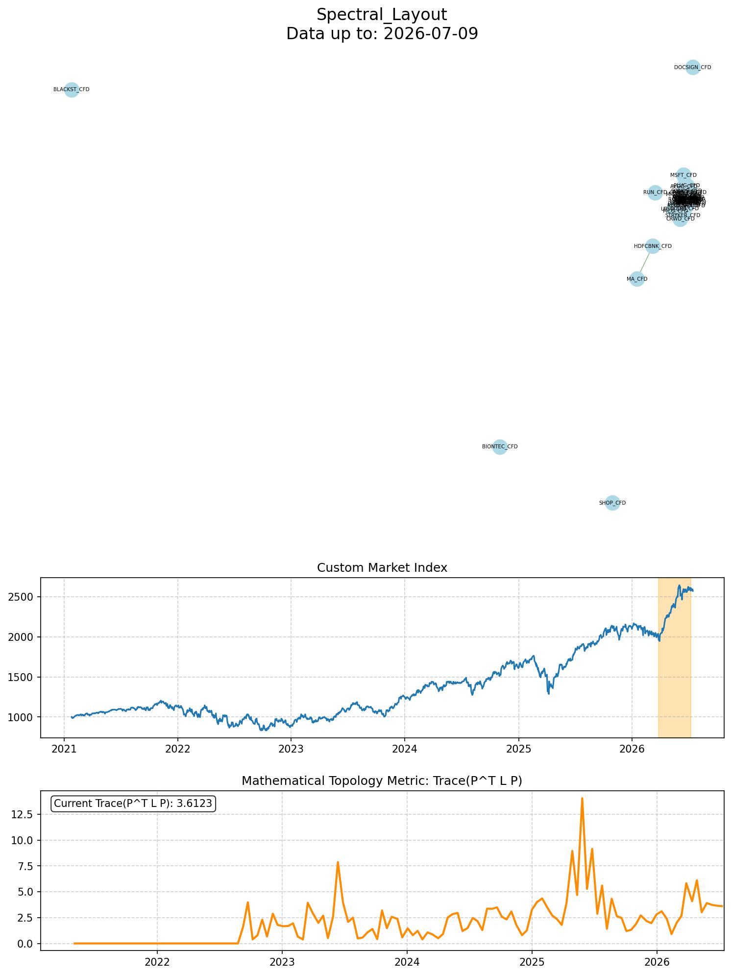
5. Trace of the Scaled Laplacian The Spectral layout finds optimal node coordinates by minimizing the trace of the position matrix scaled by the Graph Laplacian. The mathematical metric evaluated is:
\[\text{Trace} = \text{Tr}(P^T L P)\]Where:
- $P$ is the $n \times 2$ position matrix containing the $(x, y)$ coordinates of all nodes.
- $L$ is the Graph Laplacian matrix, defined as $L = D - A$.
- $D$ is the Degree Matrix and $A$ is the Adjacency Matrix.
Representation of Spectral Layout Graph
IV. Barnes-Hut Simulation
1. The Philosophy: N-Body Astrophysics and Macro Approximation The philosophy of the Barnes-Hut Simulation comes directly from astrophysics, originally designed to calculate the gravitational pull between millions of stars in a galaxy. In standard force-directed layouts (like Fruchterman-Reingold), computing the repulsion between every single pair of nodes becomes impossibly slow for massive networks. Barnes-Hut introduces a brilliant approximation: if a cluster of distant assets (a “galaxy”) is far enough away from the asset you are currently looking at, you do not need to calculate the individual repulsion of every asset in that cluster. Instead, you treat the entire cluster as a single, giant “super-node” located at its center of mass.
2. The Mathematics This approach reduces the computational complexity of calculating repulsive forces from an unscalable $O(\vert{}V\vert{}^2)$ down to a highly efficient $O(\vert{}V\vert{} \log \vert{}V\vert{})$.
It does this by partitioning the 2D space into a quadtree (recursively dividing the space into four quadrants). To decide whether to treat a distant quadrant as a single super-node or to break it open and look at the individual nodes inside, it uses a simple geometric threshold based on the width of the region ($s$) and the distance from the current node to the region’s center of mass ($d$):
\[\frac{s}{d} < \theta\]Where $\theta$ is a user-defined accuracy parameter (usually around 0.5). If the quotient is less than $\theta$, the region is far enough away to be approximated as a single point of mass.
3. The Algorithm (How It Works) Barnes-Hut acts as a drop-in acceleration engine for force-directed algorithms:
- Tree Construction: At the start of every iteration, the algorithm places all assets into a bounding box. It recursively divides this box into four smaller squares, continuing until every asset is alone in its own square. This forms the “quadtree.”
- Center of Mass Calculation: It works backwards up the tree, calculating the center of mass and total weight for every square based on the assets it contains.
- Force Approximation: When calculating the repulsive push on a specific asset, the algorithm starts at the top of the tree. It checks the $\frac{s}{d} < \theta$ condition. If true, it calculates the push using the center of mass. If false, it opens the square and repeats the check on the four smaller squares inside.
- Update and Repeat: The assets are moved based on these highly efficient approximate forces, the quadtree is destroyed, and the process repeats for the next iteration.
4. The Economic Perspective Barnes-Hut perfectly mirrors the realities of top-down portfolio management and macroeconomic scaling:
- Macro vs. Micro Focus: As an investor holding Apple, you care deeply about the specific, granular correlations to Microsoft or Google (which the algorithm calculates exactly). However, you do not need to know the specific, granular relationship between Apple and every single micro-cap mining stock in Australia. The algorithm intuitively groups those miners into a “Mining Sector Center of Mass” and calculates a single macro repulsion force against Apple.
- Massive Scalability: Standard graph layouts choke when analyzing global markets. Barnes-Hut allows quantitative analysts to map entire global equities universes (10,000+ assets) simultaneously.
- Systemic Gravity: By visualizing the “centers of mass” of different quadtree branches, analysts can see the gravitational pull of entire market sectors. A massive, heavily capitalized sector (like US Tech) acts as a dense super-node, exerting massive topological gravity that shapes the layout of emerging markets, bonds, and commodities around it.
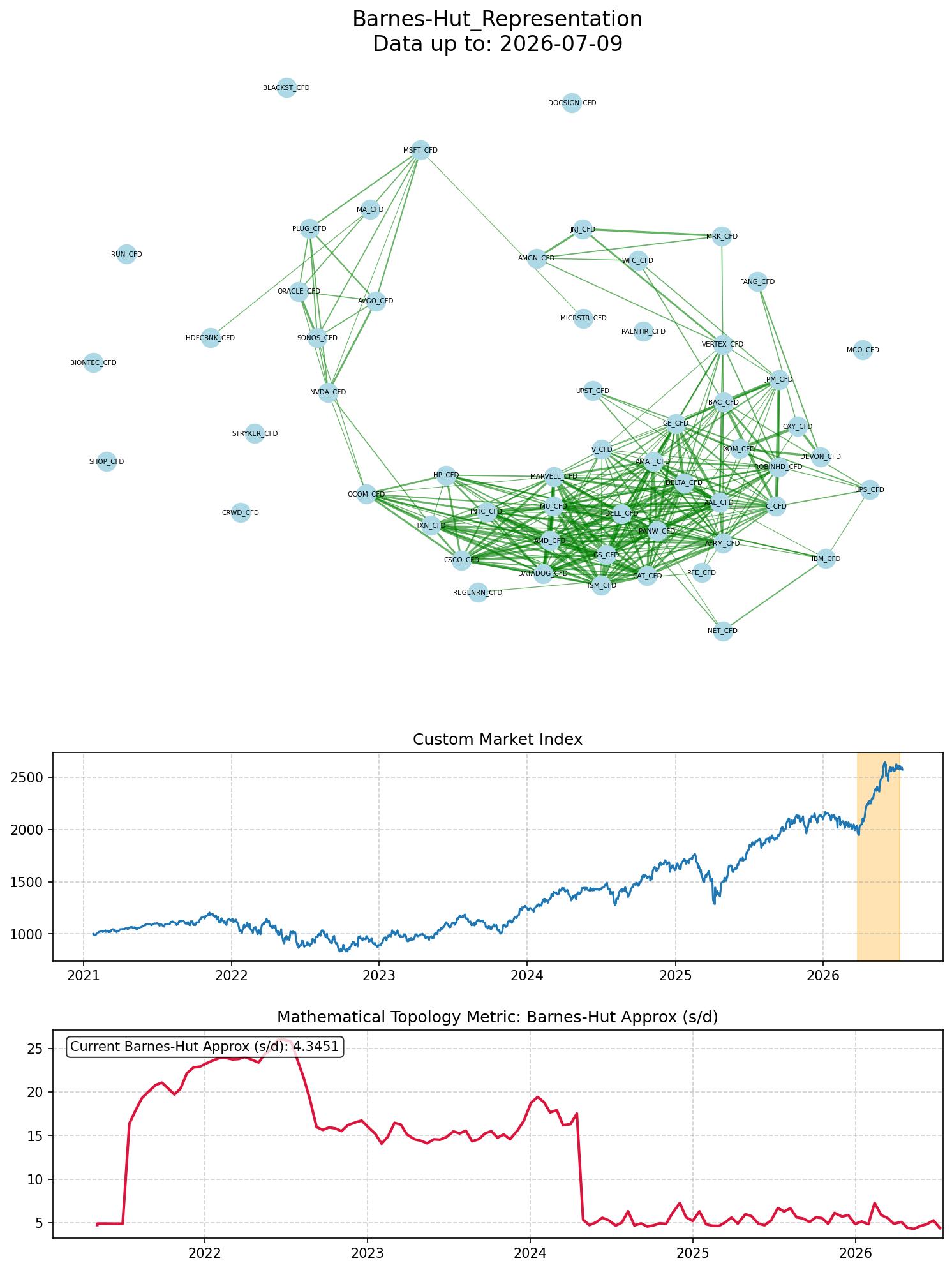
5. Force Approximation Ratio The Barnes-Hut algorithm speeds up repulsive force calculations by grouping distant nodes into “super-nodes” (centers of mass). It determines whether to approximate a cluster using the spatial ratio $\theta$:
\[\theta = \frac{s}{d}\]Where:
- $s$ is the width (size) of the bounding box containing the cluster of distant nodes.
- $d$ is the geometric distance from the target node to the cluster’s center of mass.
If $\frac{s}{d}$ is less than a predefined threshold (usually around $0.5$), the entire cluster is approximated as a single point of mass, bypassing the need for pairwise calculations.
Representation of Barnes-Hut Simulation Graph
5. Conclusion
The static mapping of financial correlation networks—whether through the physical metaphors of Fruchterman-Reingold and Barnes-Hut, the stress-minimization of Kamada-Kawai, or the algebraic decomposition of the Spectral Layout—provides a powerful, multidimensional view of market structure. However, these static representations are only the foundational step of an ongoing quantitative project.
The true value of this graph-theoretic approach lies in its temporal dynamics. As this project advances, our primary focus will shift toward analyzing how the topology of these networks changes as market time moves forward.
By applying these mapping algorithms over rolling historical time windows, we aim to capture the fluid evolution of the market. Tracking how clusters condense during liquidity crises, how peripheral safe-havens detach from the core during macroeconomic shocks, and how latent spectral factors rotate over business cycles will allow us to move beyond static visualization. Ultimately, measuring these topological shifts over time will enable us to quantify systemic risk, identify early warning signs of contagion, and build truly adaptive, structure-aware portfolios.